“Abundance distributions for tree species in Great Britain: a two-stage approach to modeling abundance using species distribution modeling and Random Forest” https://onlinelibrary.wiley.com/doi/10.1002/ece3.2661 (2016) provides predicted abundance map rasters at https://sylva.org.uk/forestryhorizons/documents/Predicted%20abundance%20map%20rasters.zip. These are relatively easy to use in QGIS.

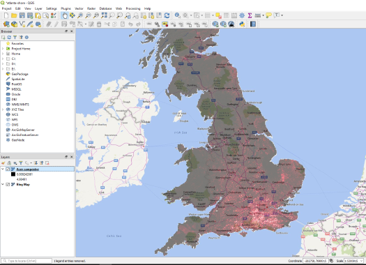
Layer > Add Layer > Add Raster Layer...

But less straight forward to display on Google Maps. Fortunately, Hollie Olmstead has done the hard work and demonstrates a solution http://zevross.com/blog/2015/08/21/process-a-raster-for-use-in-a-google-map-using-r/ using R. This is hardly surprising since if you look a the .grd files they were originally created with R package ‘raster’. The .grd header file comes with and associated .gri binary data file of the same name.

[general]
creator=R package 'raster'
created=2016-09-22 15:22:09
[georeference]
nrows=963
ncols=596
xmin=59000
ymin=13000
xmax=655000
ymax=976000
projection=+proj=tmerc +lat_0=49 +lon_0=-2 +k=0.9996012717 +x_0=400000 +y_0=-100000 +ellps=airy +datum=OSGB36 +units=m +no_defs +towgs84=446.448,-125.157,542.060,0.1502,0.2470,0.8421,-20.4894
[data]
datatype=FLT8S
byteorder=little
nbands=1
bandorder=BIL
categorical=FALSE
minvalue=4.82580326206516e-05
maxvalue=7.75424575805664
nodatavalue=-1.7e+308
[legend]
legendtype=
values=
color=
[description]
layername=AcaAbundance

The approach is to transform the raster using a coordinate reference system appropriate to Google Maps and then produce a deformed image to suit. Hollie Olmstead tries a number of different approaches. This seems the least obvious, but generates the best result.

# Load the spatial packages
library(raster)
library(rgdal) # geographical data abstraction layer

# Import the original raster and project with the new CRS
imported_raster <- raster("./acer-campestre.grd")
plot(imported_raster)
crs <- "+proj=longlat +ellps=WGS84 +datum=WGS84 +no_defs"
projected_raster <- projectRaster(imported_raster, crs=crs, method="ngb") 

# Take a look at the 
plot(projected_raster)
projected_raster
width <- 992
height <- 676

# Create an image without a background and deform to match the CRS
png(filename="./tree-map.png", bg="transparent", width=width, height=height)
par(mar = c(0,0,0,0))
raster::image(projected_raster, axes=FALSE, xlab=NA, ylab=NA)
dev.off()

Now a the image can be used in a Google Map overlay.

var treeOverlay;
function initMap() {
    var map = new google.maps.Map(document.getElementById('map'), {
    zoom: 6,
    center: {lat: 52.489471, lng: -1.898575},
    mapTypeId: google.maps.MapTypeId.TERRAIN
    });
    var bounds = {
        north: 58.7527,
        south: 49.83462,
        east: 2.470118,
        west: -7.940282
    };
    var options = {
        opacity:0.5
    }
    var image = 'https://joejcollins.github.io//assets/tree-map.png'
    treeOverlay = new google.maps.GroundOverlay(image, bounds, options);
    treeOverlay.setMap(map);
}

Producing this map.